这个分支的几篇paper倒是有点意思。我们知道，RL的很多问题中，一旦$\mathcal{P}(s|s, a), \mathcal{R}(s, a),\pi(s,a)$中有一个是non-deterministic，那么必然会使得$Q(s, a)$也应该是non-determinsitc的，而我们之前提到的算法中， DNN输出的$Q(s, a)$却是determinisitic的，那么训练中的target Q value必然会产生震荡。本节的几篇文章都是围绕着这个问题展开的。

A Distributional Perspective on Reinforcement Learning

C51的解决思路很简单。就是将$Q(s,a)$的值分布视为在$[-10, 10]$之间的51个均匀区间的categorial distribution，如此，则$Q(s,a)$的输出则为概率分布。那么这种情况下，Bellman Equation是如何实现的呢？

如果$Q^\pi(s', a')$是一个分布，那么Bellman Equation的RHS: $r(s, a) + \gamma Q^\pi(s', a')$是对原分布的变形，如原文中的下图所示:

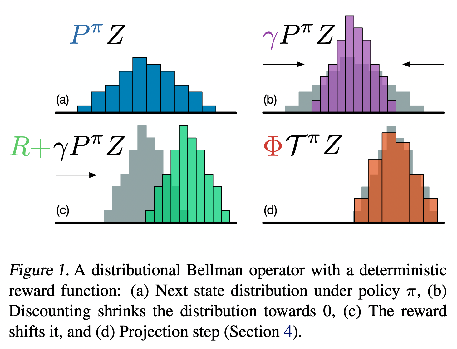
其对应的伪代码如下：

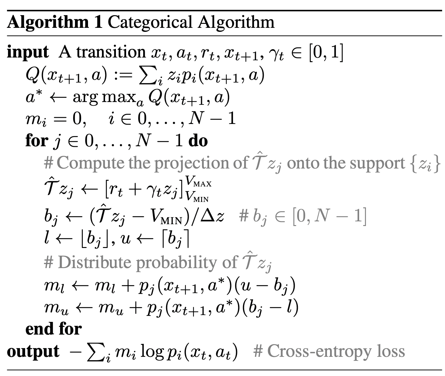
我们接下来一行一行解释以上code。首先，算法规定了$Q(s,a)$的取值范围， 比如$[-10, 10]$, 那么将这个区间平均分成50份，那么一共会有以下51个端点$\{-10, -9.6, -9.2, \dots, 9.6, 10\}=\{z_i\}$，文中被称为51个support $\{z_i\}$，这也是算法被简称为C51的由来(51 Categories)。Q Network的output dimension 由原来的$|\mathcal{A}|$变为$|\mathcal{A}|\times 51$，且对每一个action对应的$1\times 51$ array取softmax以代表categorical probability $\{p_i(s, a)\}$，如此，则$Q(s, a)=\sum_i z_i p_i(s, a)$。

我们以$r = 1, \gamma = 0.99$ 为例，$\{z_i'\}=\{\mathcal{T}z_i\} = \{[r + \gamma z_i]_{-10}^{10}\} = \{-8.9, -8.504, \dots, 9.712, 10, 10, 10\}$，这一步就是所谓的compute the projection of $\mathcal{T}z_i$ on to $z_i$。接下来，我们看看何为distribute probability of $\mathcal{T} z_i$。对于$z'_0 = -8.9$， 它在$z_2 = -9.2$与$z_3 = -8.8$之间，我们需要将$z'_0$ 对应的概率$p_0$ 分配到$z_2,z_3$上，因为$z_0'$到$z_2, z_3$的距离比为$(9.2-8.9):(8.9-8.8)=3:1$，所以将$p_0$ 的$0.25$分配到$z_2$上，$0.75$分配到$z_3$上，以此类推。然而GPU代码层面要实现以上逻辑会复杂的多，因为涉及到寻找一个batch的index的问题。

经过以上操作，Bellman Equation的RHS和LHS的categorical distribution即有相同的support, 那么两个分布之间的距离即可用cross entropy来衡量，并以此作为loss。

Distributional Reinforcement Learning with Quantile Regression

QR-DQN是在C51的基础上做了稍许改进，甚至和C51一枚硬币的两面。C51中，support是fixed and evenly distributed，Q Network输出的是support对应的probability；而在QRDQN中，probability是fixed and evenly distributed，Q Network输出的是support。

相比起C51，QR-DQN在code层面要简洁和简单很多。以作者的标准算法为例，Q Network的输出为$|\mathcal{A}| \times 200$的array，每个action对应的$1 \times 200$的array即代表quantile distribution的两百个evenly distributed quantiles $\{z_i\}$，如此则$Q(s, a) = N^{-1}\sum_{i=1}^N z_i$。

那么quantile distributions之间的loss又如何计算呢？文中的下图即是作者的思路。不同于C51中计算又相同support的categorical distribution的cross entropy，QR-DQN想要用quantile distribution去逼近return的真实distribution，计算的是两个distributions的cumulated distribution probability(CDF)之间的1-Wasserstein error。

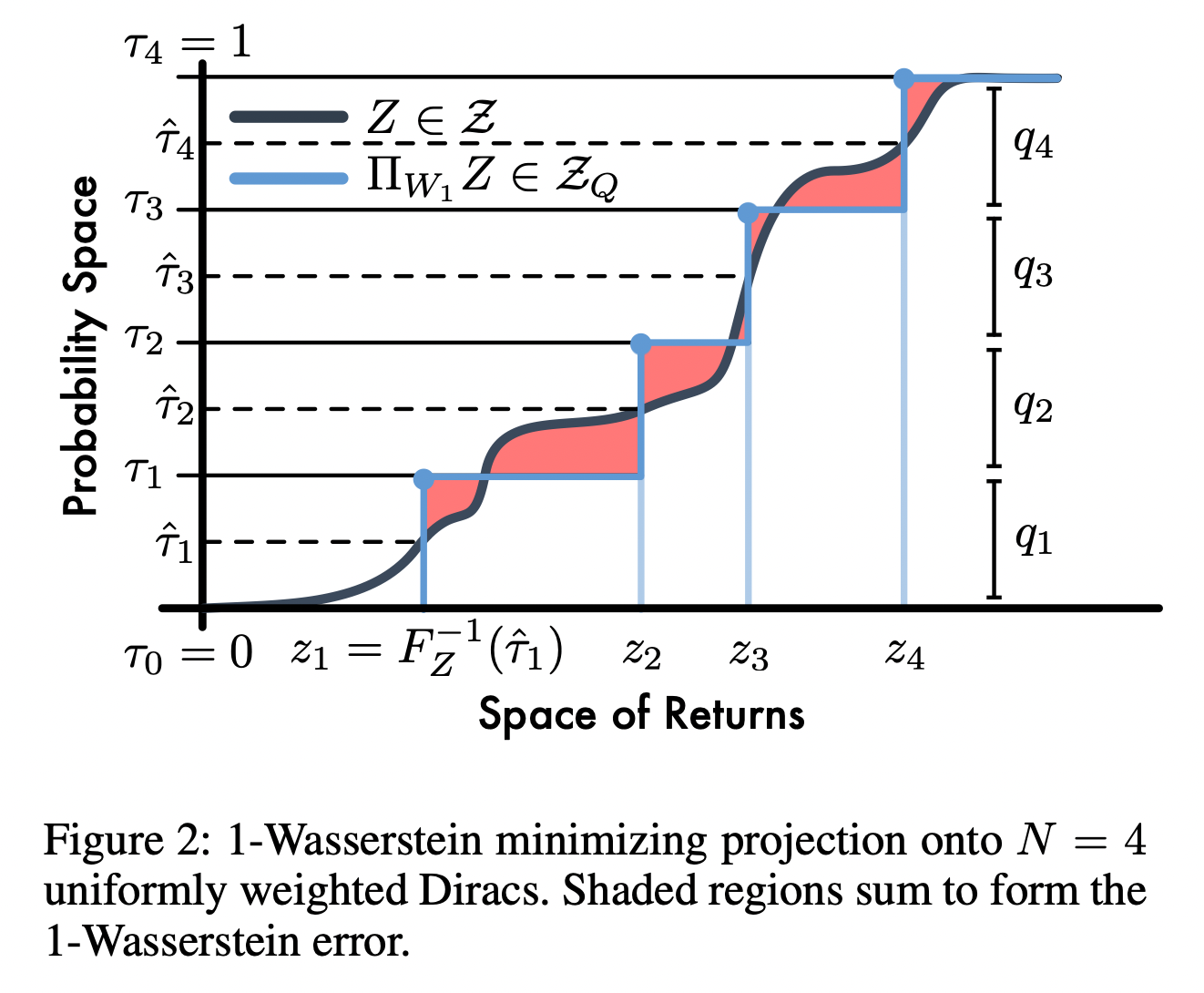
在具体计算中，作者用到了Quantile Regression的概念。所以接下来我们简单介绍下何为Quantile Regression。设random variable $Y$的cumulative distribution function为$F_Y(y) = P(Y \leq y)$，我们设分为分位数$\tau \in [0, 1]$对应的分位点为$\bar y$，则有$P(Y \leq \bar y) = \tau$，亦或者$\bar y = q(\tau) = F_Y^{-1}(\tau) = \inf \{y: F_Y(y) \geq \tau \}$。

那么问题来了，对于给定的$F_Y(y)$，如何求分位数$\tau$对应的分位点$F_Y^{-1}(\tau)$呢？我们设$L_\tau(u) = \mathbb{E}[(Y-u)(\tau-\mathbb{I}_{Y<u})]$，则

其中

我们对$L_\tau(u)$求导令其为零，则有

即$F_Y(u) = \tau, u= F^{-1}(\tau)=q(\tau)$。所以我们最小化$L_\tau(u)$，即可求得$\tau$的分位点$q(\tau)$。

如果$F_Y(y)$是quantile distribution，那么quantile regression loss为：

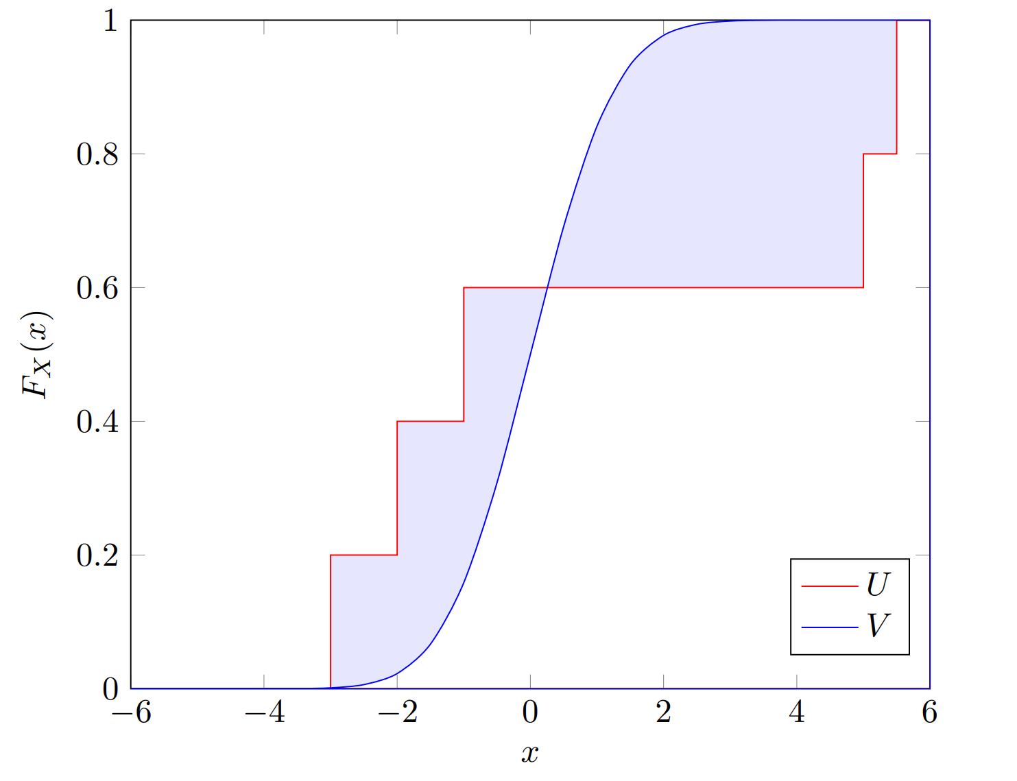
下面举例说明两个quantile distribution之间的QR loss。假设我们有quantile distribution $\mathcal{Q}=\{-5, -2, 3, 5, 8\}$ ，其对应的分位数$\tau_Q=\{0.1, 0.3, 0.5, 0.7, 0.9\}$，另有quantile distribution $\mathcal{P} = \{-3, -1, 2, 4, 7\}$ 且$\tau_P = \tau_Q$，那么$\mathcal{P, Q}$之间的Quantile Regression Loss

其对应code为

import torch
p = torch.tensor([-3, -1, 2, 4, 7])
q = torch.tensor([-5, -2, 3, 5, 8])
tau = torch.tensor([0.1, 0.3, 0.5, 0.7, 0.9])
diff = p.view(-1, 1) - q.view(1, -1)

weight = tau - (diff > 0).float()
loss = diff.abs() * weight.abs()
loss = loss.sum(-1).mean(-1)

Implicit Quantile Networks for Distributional Reinforcement Learning

IQN又在QR-DQN的基础上做了改进。我们知道，QR-DQN的分位数$\tau$是fixed and evenly distributed，所以很自然的想到，有没有办法也让$\tau$是variable？IQN的思路是在network方面动手，如文中的下图所示。

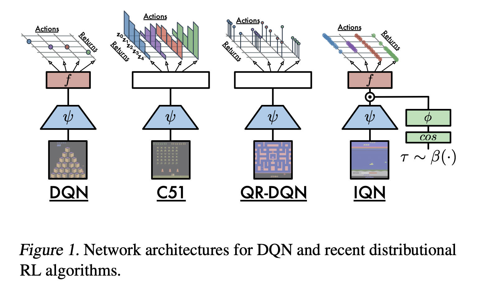
IQN的网络输入，除了RL的state之外，还有一个随机采样的分位数$\tau$，这个分位数被嵌入到网络中，并与convolution layers出来的feature互动，输出对应的分位点$q(\tau)$。

import torch
import torch.nn as nn
import numpy as np

class Network(nn.Module):
  # ......
  def forward(self, states, N):
    B = states.size(0) # Batch Size
    x = self.convs(states).view(B, -1) # convolution layers
    
    taus = torch.rand(B, N, 1) # Sample taus from uniform distribution
		pis = np.pi * torch.arange(1, self.num_cosines + 1).to(x).view(1, 1, -1)
    cosine = pis.mul(taus).cos().view(B * N, self.num_cosines)
    
    tau_embed = self.cosine_emb(cosine).view(B, N, -1)
    state_embed = x.view(B, 1, -1)
    features = (tau_embed * state_embed).view(B * N, -1)
    
    q = self.dense(features).view(B, N, -1) # B x N x |A|
    return q, taus

我在上面大概写了下算法对应的python code。网络每forward一次，便输出一个$B \times N$的$\tau$，以及与其对应的$B\times N \times |\mathcal{A}|$的quantiles，其余部分与QR-DQN相同。很多人会疑惑cosine embed这层的操作，其实这完全是调参试出来的结果，可以在Appendix里面的Figure 5看到，因为加了这个效果更好。

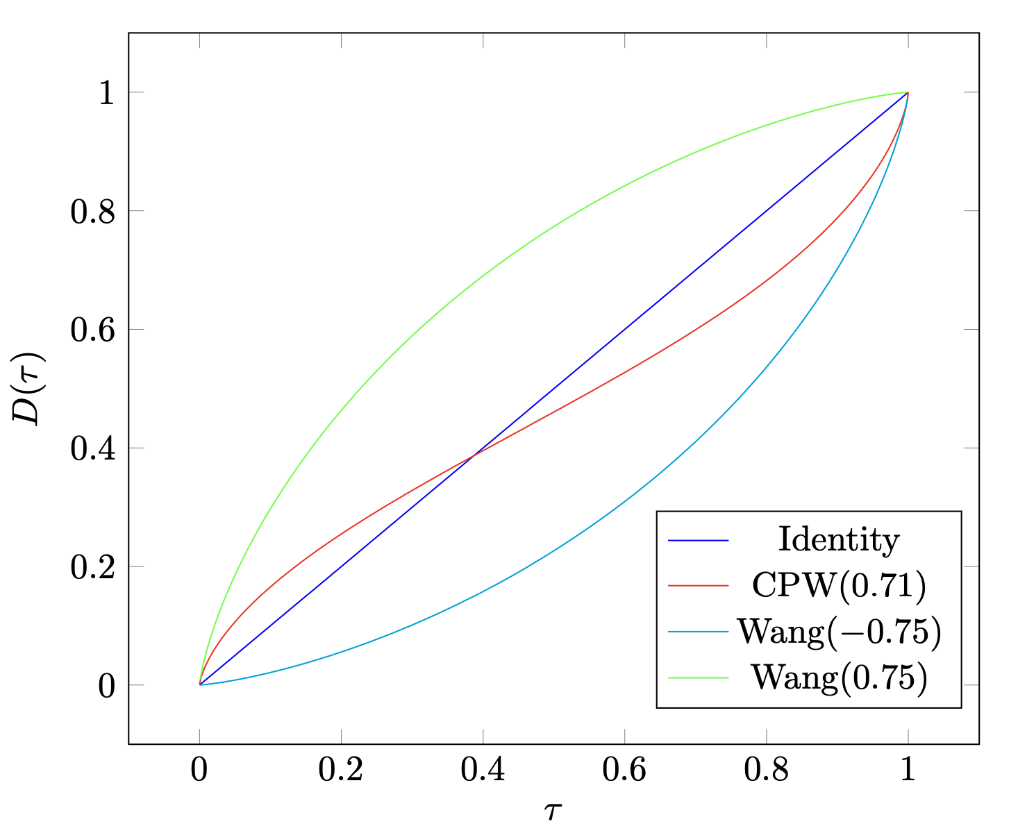
文中花了大量篇幅讲distortion risk measure，作者本期望通过distortion function来调整policy的risk偏好，结果发现还是identity distortion function，即neutral policy的总体效果最好。这里我们也简单解释下何为distortion risk measure。首先，我们需要定义一个distortion function $D:[0, 1] \rightarrow [0, 1]$，且要求$D$是continuous and increasing, 如此则$D(0) = 0, D(1) = 1$。之前我们提到，对于random variable $Y$，其CDF为$F_Y(y) = P(Y \leq y)$，quantile function为$q(\tau) = F_Y^{-1}(\tau) = \inf \{y: F_Y(y) \geq \tau \}, \tau \in [0, 1]$，那么distortion risk measure为

而我们知道

对比以上两式我们发现，本质上，distortion risk measure是在将CDF distort之后的expected 。我画出了文中提到的主要的distortion function $D(\tau)$，如下图

如果被distort的是normal distribution，那么distort之后的distribution如下

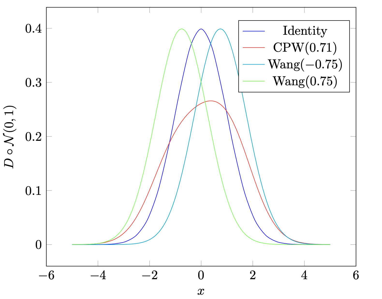
我们接着理解，为什么convex distortion function会给出risk seeking policy而concave distortion function会给出risk averse policy。我们看到，concave的$\text{Wang}(-0.75)$给出的distribution，相对于identity normal distribution而言向右移动了，也就是说，我们的policy更倾向于选higher estimated return的action（即便我们的estimation可能没那么好），而避免选择lower estimated return的action，这就是所谓的risk averse；反之，convex的$\text{Wang}(0.75)$是risk seeking，也是一样的道理。而这其实就是exploration和exploitation的问题，risk seeking policy更倾向于explore未知的领域，即便它可能带来lower return。但是基于estimated return来判断是否需要explore，这显然不太合适。

Fully Parameterized Quantile Function for Distributional Reinforcement Learning

FQF这篇文章又在IQN的基础上做了改进。我们知道，IQN的分位点$\tau$是随机采样的，FQF的想法是，$\tau$应该是根据输入的states产生的。如下图，作者认为，相比于随机采样的$\tau$，显然经过调整的$\tau$会使得1-Wasserstein的loss更小。

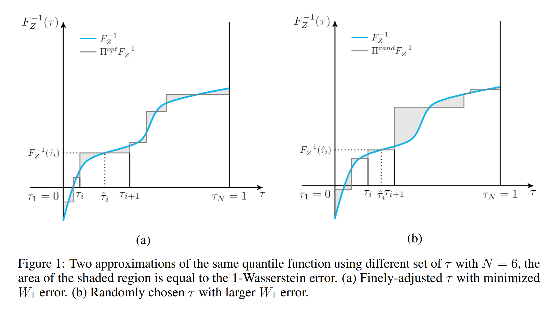
所以接下来要回答的问题是，如何调整$\tau$。要回答这个问题，需要系统的了解下Wasserstein Distance。

For two distrubtions $U, V$, their Wasserstein Distance is given by:

$$W_p(U, Y) = (\int_0^1|F_Y^{-1}(\omega) - F_U^{-1}(\omega)|^pd\omega)^{1/p}$$

where $F_Y^{-1}(\omega)$ is the inverse CDF of distrubtion $Y$, which means $F^{-1}_Y(\omega) := \inf\{y\in \mathbb{R}: \omega \leq F_Y(y) \}$

Inverse CDF这里解释的有点绕口，我们知道CDF是PDF(Probability Density Function)的积分: $F_Y(y) = \int_{-\infty}^{\infty}f(y)dy$，Inverse CDF就是CDF的反函数。在下图中：

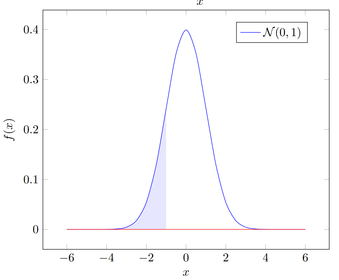
$f(x) = \mathcal{N}(0,1)$ 为standard normal distribtuion，涂色面积$\omega$，那么 $F_X^{-1}(\omega) = -1$。

特殊情况下，如果$U = \{\theta_1, \dots, \theta_N\}$是quantile distribution with $\{\tau_i\}=\{F_U(\theta_i)\}, \tau_0 = 0, p=1$,那么

如下图的CDF，其中$U=\{(\tau_i, \theta_i)\}$ with $\{\theta_i\} = \{-3, -2, -1, 5, 5.5\}, \{\tau_i\} = \{0.2, 0.4, \dots, 1.0\}, \tau_0 = 0$ and $V=\mathcal{N}(0, 1)$，涂色部分的面积即为$W_1(U, V)$。

问题又来了，如果quantile distribution $U$ 的 support $\{\theta_i\}$是可调节的，那么如何才能使$W_1$最小呢？

For any $\tau, \tau' \in [0, 1]$ and $\tau < \tau'$, and CDF $F$ with its inverse $F^{-1}$, the set of $\theta \in \mathbb{R}$ minimizing

$$L(\theta) = \int_{\tau}^{\tau'} |F^{-1}(\omega) - \theta| d\omega$$

is given by

$$\{\theta \in \mathbb{R} | F(\theta) = \frac{\tau + \tau'}{2}\}$$

Or

$$\arg\min L(\theta) = F^{-1}(\frac{\tau+\tau'}{2})$$

这部分其实很好证明。首先，显然$L(\theta|F(\theta) < \tau) > L(\theta|F(\theta) = \tau), L(\theta|F(\theta) > \tau') > L(\theta|F(\theta) = \tau')$，所以$\arg\min_\theta L(\theta) \in [F^{-1}(\tau), F^{-1}(\tau')]$，那么

那么对于上面提到的quantile distribution $U$ with quantile fractions $\{\tau_0, \dots, \tau_N\}$ and $\tau_0 = 0, \tau_N = 1, \tau_i \leq \tau_{i+1}$ 和 continuous distribution $V$,

我们设$\hat{\tau}_i = (\tau_i + \tau_{i-1})/2$，那么

我们又设 $L(\tau_i) = \min W_1(U, V)$，那么

上式的证明可参考文章的Appendix，也是FQF算法的核心结论。另外，很容易推出

文章其他部分与IQN相同。我这里摘抄对应的code方便解释。

class Network(nn.Module)
  ...

  def taus_prop(self, x):
    batch_size = x.size(0)
    log_probs = self.fraction_net(x).log_softmax(dim=-1) # Faction Network: B X F => B X P
    probs = log_probs.exp()
    tau0 = torch.zeros(batch_size, 1).to(x)
    tau_1n = torch.cumsum(probs, dim=-1)

    taus = torch.cat((tau0, tau_1n), dim=-1) # B X (P + 1)
    taus_hat = (taus[:, :-1] + taus[:, 1:]).detach() / 2.0 # B X P
    entropies = probs.mul(log_probs).neg().sum(dim=-1, keepdim=True)
    return taus.unsqueeze(-1), taus_hat.unsqueeze(-1), entropies
  
  def calc_fqf_q(self, x):
    if st.ndim == 4:
        convs = self.convs(st)
    else:
        convs = st
    # taus: B X (N+1) X 1, taus_hats: B X N X 1
    taus, tau_hats, _ = self.taus_prop(convs.detach())
    q_hats, _ = self.forward(convs, taus=tau_hats)
    q = ((taus[:, 1:, :] - taus[:, :-1, :]) * q_hats).sum(dim=1)
    return q

  def forward(self, x, taus_hat=None):
    B = states.size(0) # Batch Size
    x = self.convs(states).view(B, -1) # convolution layers, output x: B X F
    
    if taus_hat is None:
      _, taus_hat, _ = self.taus_prop(x.detach())
    
    N = taus_hat.size(1)

    ipi = np.pi * torch.arange(1, self.cfg.num_cosines + 1).to(x).view(1, 1, self.cfg.num_cosines)
    cosine = pis.mul(taus_hat).cos().view(B * N, self.num_cosines)
    
    tau_embed = self.cosine_emb(cosine).view(B, N, -1)
    state_embed = x.view(B, 1, -1)
    features = (tau_embed * state_embed).view(B * N, -1)
    
    q = self.dense(features).view(B, N, -1) # B x N x |A|
    return q, taus_hat

class Agent:
  ...

  def step(self, states, next_states, actions, terminals, rewards):
    q_convs = self.model.convs(states)
    taus, tau_hats, _ = self.model.taus_prop(q_convs.detach())
    # q_hat: B X N X A
    q_hat, _ = self.model.forward(q_convs, taus_hat=tau_hats)
    q_hat = q_hat[self.batch_indices, :, actions]

    with torch.no_grad():
      q_next_convs = self.model_target.convs(next_states)
      q_next_ = self.model_target.calc_fqf_q(q_next_convs)
      a_next = q_next_.argmax(dim=-1)

      q_next, _ = self.model_target.forward(q_next_convs, taus=tau_hats)
      q_next = q_next[self.batch_indices, :, a_next]
      q_target = rewards.unsqueeze(-1).add(
        self.cfg.discount ** self.cfg.n_step * (1 - terminals.unsqueeze(-1)) * q_next)

    q_current_, q_target_ = q_hat..unsqueeze(1), q_target.unsqueeze(-1)
    diff = q_hat.unsqueeze(1) - q_target.unsqueeze(-1)
    # q_current_: B X 1 X N
    # tau_hats: B X 1 X N
    # q_target_: B X N X 1
    loss = nn.functional.smooth_l1_loss(diff) * (taus_hat - q_target.lt(q).detach().float()).abs()

    # Calculate Fraction Loss
    with torch.no_grad():
      q, _ = self.model.forward(q_convs, taus_hat=taus[:, 1:-1])
      q = q[self.batch_indices, :, actions]
      values_1 = q - q_hat[:, :-1]
      signs_1 = q.gt(torch.cat((q_hat[:, :1], q[:, :-1]), dim=1))

      values_2 = q - q_hat[:, 1:]
      signs_2 = q.lt(torch.cat((q[:, 1:], q_hat[:, -1:]), dim=1))
    gradients_of_taus = (torch.where(signs_1, values_1, -values_1) + torch.where(signs_2, values_2, -values_2)
      ).view(self.cfg.batch_size, self.cfg.N_fqf - 1)
    fraction_loss = (gradients_of_taus * taus[:, 1:-1, 0]).sum(dim=1).view(-1)

计算Faction Loss之前其实很好懂，相当于用fraction network产生的$\{\hat{\tau}_i\}$代替随机生成的，所以我们着重理解Calculate Fraction Loss这部分，对照着$\partial L(\tau_i) /\partial \tau_i$其实很好理解。

q其实在计算$F^{-1}_V(\tau_i)$，q_hat[:, :1]和q_hat[:,1:]对应的是$F^{-1}_V(\hat{\tau}_{i-1})$和$F^{-1}_V(\hat{\tau}_{i})$，gradients_of_taus计算的是

到这里大家可能会疑惑为何不套用解开绝对值之后的公式，原因很简单，因为我们的neural network计算出来的$F_V^{-1}$并不是严格的non-decreasing，直接套用会导致梯度计算并不准确。为了解决这一问题，后续有作品提出non-decreasing quantile network，这里就不多说了。