我们现实中的很多问题，都可以归纳为图搜索问题，因此它在地图导航，路径规划，游戏AI中得到广泛的应用。而我们在动态规划里面提到的几个问题，其实是图搜索问题的几个特例。这也使得我们有必要单独写一篇介绍这一类问题的算法。

Graph search, also known as graph traversal, refers to the process of visiting each vertex in a graph. Graphs have nodes and edges $G = <V, E>$ . Edges can be directed or undirected, weighted or unweighted.

本文将以此介绍一下几个算法:

深度优先搜索 Depth First Search

我们以下图为例

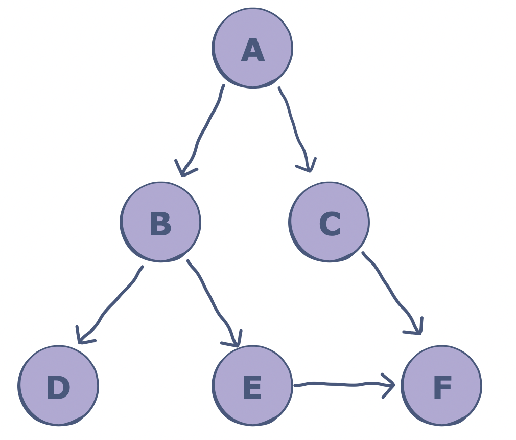
graph = {
    'A' : ['B','C'],
    'B' : ['D', 'E'],
    'C' : ['F'],
    'D' : [],
    'E' : ['F'],
    'F' : []
}

visited = set() # Set to keep track of visited nodes.

def dfs(visited, graph, node):
    if node not in visited:
        print(node)
        visited.add(node)
        for neighbour in graph[node]:
            dfs(visited, graph, neighbour)

dfs(visited, graph, 'A')

运行的结果是

A
B
D
E
F
C

广度优先搜索 Breadth First Search

同样以上图为例

visited = []   # List to keep track of visited nodes.
queue = []     # Initialize a queue

def bfs(visited, graph, node):
  visited.append(node)
  queue.append(node)

  while queue:
    s = queue.pop(0) 
    print(s) 

    for neighbour in graph[s]:
      if neighbour not in visited:
        visited.append(neighbour)
        queue.append(neighbour)

# Driver Code
bfs(visited, graph, 'A')

运行的结果是

A
B
C
D
E
F

我们很容易发现，深度优先算法找到的路径并不是最短路径，而广度优先回溯出来的的才是。后面介绍的Dijkstra's Algorithm和A* Algorithm就是基于BFS的算法。

戴克斯特拉算法 Dijkstra's Algorithm

BFS与其说是找的最短路径，不如说是找的最少途径点，因为graph中所有的edge权值相等。这就导致了其应用的局限性。现实中，比如城市中两地间的交通，距离路况等等，都影响我们的选择，这时候BFS就不适用了。

我们以下图为例:

要求从 $a$ 点出发，找到其他所有点到 $a$ 点的最优路径，我们设 $N(x)$ 为 $x$ 的邻点。

数组 $D = [\infty, \infty, \infty, \infty, \infty, \infty]$ 已记录的 $a$ 到 $a,b,c,d,e,f$ 的最优距离；
集合 $V = \empty$ , 代表已经访问过的节点。
集合 $S = \{a\}$ , 代表正在访问的节点。

\begin{array}{c|l|l} \textrm{Step} & \\ \hline 1 & \textrm{State} & S = \{a\}, D = [0, \infty, \infty, \infty, \infty, \infty], V = \emptyset \\ & \textrm{Update} & N(a) = \{b, c\}, D(b) = 10, D(c) = 20 \\ & & V = \{a\}, S = \{b, c\} \\ \hline 2 & \textrm{State} & S = \{b, c\}, D = [0, 10, 20, \infty, \infty, \infty], V = \{a\} \\ & \textrm{Update} & N(b) = \{e, d\}, D(e) = D(b) + 10 = 20, D(d)=D(b) + 50 = 60 \\ & & V = \{a, b\}, S = \{c, e, d\} \\ \hline 3 & \textrm{State} & S = \{c, e, d\}, D=[0, 10, 20, 60, 20, \infty], V=\{a,b\} \\ & \textrm{Update} & N(c)=\{d, e\}, D(ace)=D(c) + 33 > D(e) \\ & & D(acd) = D(c) + 20 = 40 <D(d), D(d)=40\\ & & V = \{a, b, c\}, S = \{e, d, f\} \\ \hline 4 & \textrm{State} & S = \{e, d, f\}, D = [0, 10, 20, 40, 20, \infty], V = \{a, b, c\} \\ & \textrm{Update} & N(a) = \{b, c\}, D(b) = 10, D(c) = 20 \\ & & V = \{a\}, S = \{b, c\} \\ \hline 5 & \textrm{State} & S = \{d, f\}, D = [0, 10, 20, 40, 20, 21], V = \{a, b, c, e\} \\ & \textrm{Update} & N(d) = \{e, f\}, D(ade) = D(d) + 20 > D(e) \\ & & D(adf) = D(d) + 2 > D(f) \\ & & V = \{a, b, c, e, d\}, S = \{f\}\\ \hline 6 & \textrm{State} & S = \{f\}, D = [0, 10, 20, 40, 20, 21], V = \{a, b, c, e, d\} \\ & \textrm{Update} & N(f) = \empty, V = \{a, b, c, e, d, f\}, S = \emptyset \end {array}

from collections import defaultdict

graph = {
    'a': {'c': 20, 'b': 10},
    'b': {'e': 10, 'd': 50},
    'c': {'e': 33, 'd': 20},
    'd': {'e': 20, 'f': 2},
    'e': {'f': 1},
    'f': {}
}

def dijkstra(g, s):
    D = defaultdict(lambda: float('inf'))
    P = {}
    S = [s]
    V = {}
    D[s] = 0
    
    while len(S) > 0:
        node = S.pop(0)
        for v in g[node]:
            if v not in D or D[node] + g[node][v] < D[v]:
                D[v] = D[node] + g[node][v]
                P[v] = node
            if v not in V:
                S.append(v)
        V[node] = 0
    print(D)
    print(P)

dijkstra(graph, 'a')

A*算法 A-Star Algorithm

很显然，随着节点数目的增多，Dijkstra算法需要考察的节点数目从起点层层往外增加。如果平均每个节点的子节点数目为 $N$ ，节点总数为 $M$ 的话，那么算法的平均搜索深度为 $O(\log_N M)$ ，在最深处，需要考察的节点数目为 $O(M)$ 。为了提高其搜索效率，有算法提出从起点和终点同时搜索，这其实相当于给搜索指定了方向。所以更聪明的算法呼之欲出，即本文的主角A*算法。

A* 算法是一种启发式搜索算法，所谓启发式，其实是在评估路径的时候用了一个启发函数 $h(x)$ ，A算法对节点 $x$ 的评估函数

f(x) = g(x) + h(x)

这里 $g(x)$ 是起点到节点 $x$ 的最优距离，即上文中Dijkstra算法中的 $D(x)$ , $h(x)$ 是对节点 $x$ 到目标节点的估算距离。A*算法会优先考察 $f(x)$ 最小的节点。值得注意的是：

如果 $g(x)$ , 本算法即为最佳搜索优先算法BFS，速度最快，但解不是最优。
如果 $h(x)$ , 本算法即为Dijkstra算法，计算的节点最多。
$h(x)$ 的选取，常用的有欧式距离(L2)和曼哈顿距离(L1)。

因为算法对 $h(x)$ 的需要，这也使得A*更适合在有障碍物的网格类问题中得到应用。

import numpy as np
from collections import defaultdict

class AStar:
    def __init__(self):
        self.H = 30
        self.W = 30
        self.S = (15, 17)
        self.T = (15, 25)
        graph = np.chararray((self.H, self.W))
        graph[:, :] = '.'
        graph[5:25, 20] = 'H'
        graph[5, 10:20] = 'H'
        graph[25, 10:21] = 'H'
        graph[self.S] = 'S'
        graph[self.T] = 'T'
        self.g = graph

    def distance(self, x, y):
        return np.abs(x[0] - y[0]) + np.abs(x[1] - y[1])

    def neighbors(self, node):
        x, y = node
        offset = [(-1, 0), (1, 0), (0, 1), (0, -1)]
        out = []
        for dx, dy in offset:
            ix, iy = x+dx, y+dy
            if 0 <= ix < self.H and 0 <= iy < self.H:
                if self.g[ix, iy].decode('utf-8') != 'H': 
                    out.append((ix, iy))
        return out

    def tostring(self, g=None):
        if g is None:
            g = self.g
        out = ""
        for i in range(self.H):
            out += " ".join([str(x, encoding='utf-8') for x in g[i]])
            out += '\n'
        return out

    def solve(self):
        print("Astar Path Finding")
        print("H standds for wall, S stands for source, T stands for target")
        print(self.tostring())
        D = defaultdict(lambda: float('inf'))
        D[self.S] = 0
        P = {}
        S = {self.S: 0}
        V = {}

        count = 0
        while self.T not in S:
            node = min(S, key=S.get)
            if node == self.T:
                break
            for v in self.neighbors(node):
                if v not in D or D[v] > D[node] + 1:
                    D[v] = D[node] + 1
                    P[v] = node
                    if v not in V:
                        S[v] = D[v] + self.distance(v, self.T)
            V[node] = 0
            del S[node]

        print("Finding path ...")
        print()
        print()
        print('Path found, represented by *')
        gx = np.copy(self.g)
        v = self.T
        while v in P:
            v = P[v]
            gx[v] = '*'
        
        # for k in S: gx[k] = 'O'
        # for k in V: gx[k] = 'X'
        print(self.tostring(gx))
            

s = AStar()
s.solve()

运行的结果如下:

Astar Path Finding
H standds for wall, S stands for source, T stands for target
. . . . . . . . . . . . . . . . . . . . . . . . . . . . . .
. . . . . . . . . . . . . . . . . . . . . . . . . . . . . .
. . . . . . . . . . . . . . . . . . . . . . . . . . . . . .
. . . . . . . . . . . . . . . . . . . . . . . . . . . . . .
. . . . . . . . . . . . . . . . . . . . . . . . . . . . . .
. . . . . . . . . . H H H H H H H H H H H . . . . . . . . .
. . . . . . . . . . . . . . . . . . . . H . . . . . . . . .
. . . . . . . . . . . . . . . . . . . . H . . . . . . . . .
. . . . . . . . . . . . . . . . . . . . H . . . . . . . . .
. . . . . . . . . . . . . . . . . . . . H . . . . . . . . .
. . . . . . . . . . . . . . . . . . . . H . . . . . . . . .
. . . . . . . . . . . . . . . . . . . . H . . . . . . . . .
. . . . . . . . . . . . . . . . . . . . H . . . . . . . . .
. . . . . . . . . . . . . . . . . . . . H . . . . . . . . .
. . . . . . . . . . . . . . . . . . . . H . . . . . . . . .
. . . . . . . . . . . . . . . . . S . . H . . . . T . . . .
. . . . . . . . . . . . . . . . . . . . H . . . . . . . . .
. . . . . . . . . . . . . . . . . . . . H . . . . . . . . .
. . . . . . . . . . . . . . . . . . . . H . . . . . . . . .
. . . . . . . . . . . . . . . . . . . . H . . . . . . . . .
. . . . . . . . . . . . . . . . . . . . H . . . . . . . . .
. . . . . . . . . . . . . . . . . . . . H . . . . . . . . .
. . . . . . . . . . . . . . . . . . . . H . . . . . . . . .
. . . . . . . . . . . . . . . . . . . . H . . . . . . . . .
. . . . . . . . . . . . . . . . . . . . H . . . . . . . . .
. . . . . . . . . . H H H H H H H H H H H . . . . . . . . .
. . . . . . . . . . . . . . . . . . . . . . . . . . . . . .
. . . . . . . . . . . . . . . . . . . . . . . . . . . . . .
. . . . . . . . . . . . . . . . . . . . . . . . . . . . . .
. . . . . . . . . . . . . . . . . . . . . . . . . . . . . .

Finding path ...

Path found, represented by *
. . . . . . . . . . . . . . . . . . . . . . . . . . . . . .
. . . . . . . . . . . . . . . . . . . . . . . . . . . . . .
. . . . . . . . . . . . . . . . . . . . . . . . . . . . . .
. . . . . . . . . . . . . . . . . . . . . . . . . . . . . .
. . . . . . . . . * * * * * * * * * * * * * . . . . . . . .
. . . . . . . . . * H H H H H H H H H H H * . . . . . . . .
. . . . . . . . . * * * * * * * * * . . H * . . . . . . . .
. . . . . . . . . . . . . . . . . * . . H * . . . . . . . .
. . . . . . . . . . . . . . . . . * . . H * . . . . . . . .
. . . . . . . . . . . . . . . . . * . . H * . . . . . . . .
. . . . . . . . . . . . . . . . . * . . H * . . . . . . . .
. . . . . . . . . . . . . . . . . * . . H * . . . . . . . .
. . . . . . . . . . . . . . . . . * . . H * . . . . . . . .
. . . . . . . . . . . . . . . . . * . . H * . . . . . . . .
. . . . . . . . . . . . . . . . . * . . H * . . . . . . . .
. . . . . . . . . . . . . . . . . * . . H * * * * T . . . .
. . . . . . . . . . . . . . . . . . . . H . . . . . . . . .
. . . . . . . . . . . . . . . . . . . . H . . . . . . . . .
. . . . . . . . . . . . . . . . . . . . H . . . . . . . . .
. . . . . . . . . . . . . . . . . . . . H . . . . . . . . .
. . . . . . . . . . . . . . . . . . . . H . . . . . . . . .
. . . . . . . . . . . . . . . . . . . . H . . . . . . . . .
. . . . . . . . . . . . . . . . . . . . H . . . . . . . . .
. . . . . . . . . . . . . . . . . . . . H . . . . . . . . .
. . . . . . . . . . . . . . . . . . . . H . . . . . . . . .
. . . . . . . . . . H H H H H H H H H H H . . . . . . . . .
. . . . . . . . . . . . . . . . . . . . . . . . . . . . . .
. . . . . . . . . . . . . . . . . . . . . . . . . . . . . .
. . . . . . . . . . . . . . . . . . . . . . . . . . . . . .
. . . . . . . . . . . . . . . . . . . . . . . . . . . . . .